Efficient data loading for beginners

Data loading

In essence, data loading entails reading data from persistent memory in a disk periphery, transforming the data, synchronizing the data to the GPU, and supplying it to a computation graph. In the most simplistic form, these steps are executed in sequence. This means data transformation for an arbitrary timestamp t happens first prior to the result of transformation being synchronized to the GPU over an interconnect port. This beginner tutorial assumes that you have already copied data to an ephemeral PVC mount. Because a persistent PVC mount resides at a networked file location, we do not recommend loading data from there due to the incurred networking latency. Sequential data loading can be implemented in PyTorch with the torch.utils.data.Dataset and torch.utils.data.DataLoader classes. While the Dataset class implements the methods for instantiating, reading, and transformation, DataLoader controls the behavior of a PySeqIter_Type class. An example Dataset and DataLoader implementation, including an illustration visualising the timing behavior, can be found below:

import os
import pandas as pd
import torch.nn.functional as F
from torchvision.transforms import v2
from torchvision.io import decode_image
from torch.utils.data import DataLoader

class CustomImageDataset(Dataset):

  def __init__(self, annotations_file, img_dir, transform=None, label_transform=None):

    # Two-columns: string <FILENAME>.<EXT>, int label
    self.img_labels = pd.read_csv(annotations_file)

    self.img_dir = img_dir

    # Callable types returning torch.Tensor
    self.transform = transform
        self.label_transform = label_transform

    def __len__(self):
        return len(self.img_labels)

    def __getitem__(self, idx):
        img_path = os.path.join(self.img_dir, self.img_labels.iloc[idx, 0])

    image = decode_image(img_path)
        label = self.img_labels.iloc[idx, 1]

    if self.transform:
            image = self.transform(image)
        if self.label_transform:
            label = self.label_transform(label)

    return image, label

training_data = CustomImageDataset("labels_train.csv", "labels_train/", v2.compose([..., ...]), F.one_hot)
test_data = CustomImageDataset("labels_test.csv", "labels_test/", v2.compose([..., ...]), F.one_hot)

train_dataloader = DataLoader(training_data, batch_size=64, shuffle=True)
test_dataloader = DataLoader(test_data, batch_size=64, shuffle=True)

train_batch = next(iter(train_dataloader))
test_batch = next(iter(test_dataloader))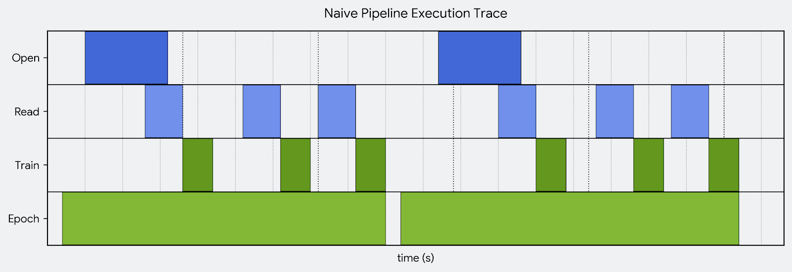

Time complexity of data loading when naively executing loading, transformation, synchronization, and supply in sequence.

In the naive sequential implementation like the one above, while loading is taking place, your graph is sitting idle. Conversely, while your graph is training, the loader is sitting idle. The training step time is thus the sum of loading, transformation, synchronization, and supply times.

DataLoader configurations

The following configuration options, among other options, are available in order to change the time and memory complexity behavior of the eventual PySeqIter_Type class:

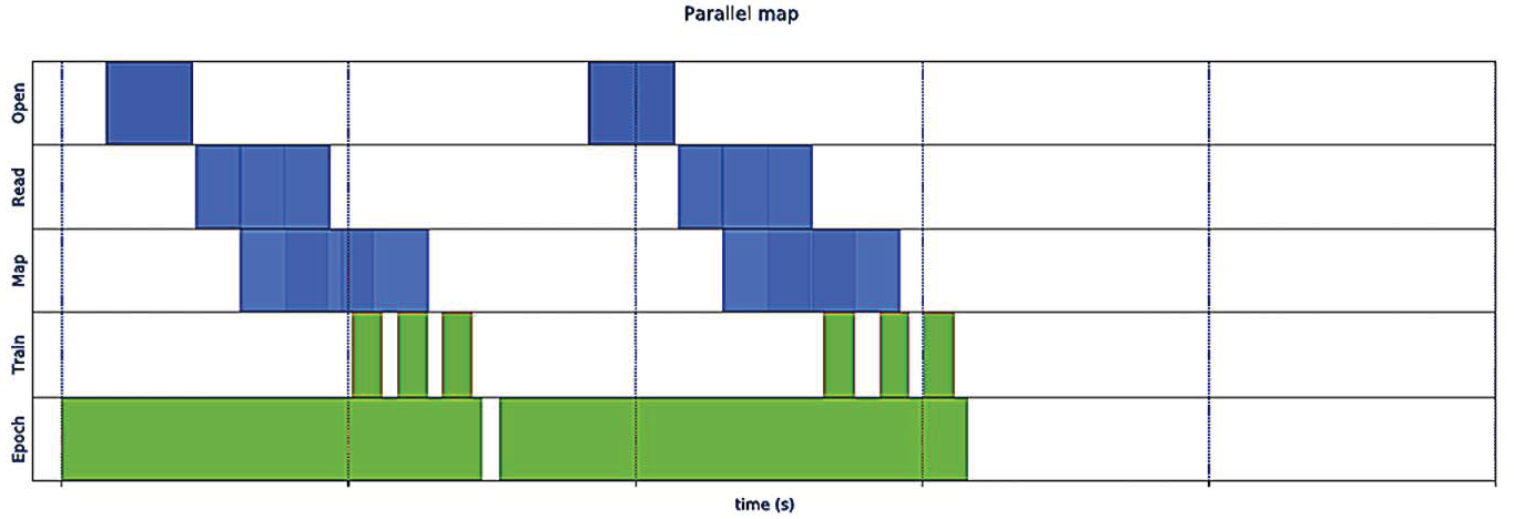
# The included values denote default DataLoader values
batch_size: int | None = 1,
in_order: bool = True,
persistent_workers: bool = False,
drop_last: bool = False,
prefetch_factor: int | None = None,
num_workers: int = 0

A larger batch size forces the memory complexity of the computation graph to increase because more data has to be transported through the graph at a single timestamp. Ordering requires additional operations for ordered handoff to the interconnect port for synchronization based on sequence index, especially when the DataLoader is asked to perform parallel loading. Persistent workers do not incur additional initialization time at the end of every epoch. When drop_last is false, there is a chance that the size of a dataset cannot be divided to a nearest integer based on the used batch size. This forces TorchDynamo to perform a costly computation graph recompilation step when the last encountered batch size is not equal to the earlier used batch size. When prefetch_factor is set, a queue is used to host batches to be synchronized to the GPU. While loading and transforming the batch for timestamp t+1, synchronization happens in parallel for timestamp t. This is typically referred to as pipelining. When num_workers is set, multiple processes simultaneously load and transform batches. Provided that the prefetch queue size is tuned effectively, the time for loading and transforming a particular batch on average decreases. The effect this has on time complexity can be found inside the image below (please be advised that map refers to applying a transformation in parallel):

Time complexity of data loading with optimized loading, transformation, synchronization, and supply pipelined and parallelized.

Configuration options can be added to the DataLoader class when instantiating the DataLoader object. The DataLoader object can subsequently be used inside a training loop where the computation graph is used for parameter training and gathering performance metric values.

Efficient data formats

For information regarding efficient data formats which can be used in machine learning pipelines, we refer to the following Surf tutorial.